Generalization to Ductile Fracture

Learning objectives

By the end of this lesson, you should be able to:

Explain the difference between brittle and ductile fracture.
Understand why Griffith fracture must be generalized for ductile materials.
Identify the role of plastic deformation in ductile fracture.
Explain how plastic work, hardening, and void growth contribute to fracture.
Understand how phase-field fracture can be coupled to elastoplasticity.
Distinguish between brittle crack surface energy and ductile fracture dissipation.
Recognize the role of stress triaxiality and Lode angle in ductile failure.
Write a conceptual phase-field energy functional for ductile fracture.

1. Brittle fracture versus ductile fracture

Fracture can occur in different ways depending on the material and loading conditions.

Two important idealized types are:

Brittle fracture
Ductile fracture

Brittle fracture

Brittle fracture occurs with little or no plastic deformation.

Examples include:

glass,
ceramics,
brittle rocks,
some polymers at low temperature,
ice under some conditions.

In brittle fracture, the main energetic cost is creating new crack surface.

The Griffith criterion is:

\[ G \geq G_c \]

where:

\(G\) is the energy release rate,
\(G_c\) is the critical fracture energy.

Ductile fracture

Ductile fracture occurs after significant plastic deformation.

Examples include:

metals,
many alloys,
ductile polymers,
some geomaterials under high confinement.

In ductile fracture, energy is not only spent creating new surfaces. A large amount of energy may be dissipated through plastic deformation.

Therefore, ductile fracture is governed by both:

\[ \text{plasticity} \]

and

\[ \text{fracture} \]

2. Why Griffith theory is not enough for ductile fracture

Classical Griffith fracture assumes that the main energy cost is the creation of crack surface:

\[ G_c |\Gamma| \]

The sharp-crack Griffith energy is:

\[ \Pi(u,\Gamma) = \int_{\Omega \setminus \Gamma} \psi_e(\varepsilon(u))\,d\Omega + G_c|\Gamma| - W_{\text{ext}}(u) \]

This is appropriate for brittle elastic fracture.

However, ductile fracture involves additional mechanisms:

plastic yielding,
plastic hardening,
void nucleation,
void growth,
void coalescence,
shear localization,
necking,
large deformation,
stress-state-dependent damage.

Therefore, for ductile fracture, the energy balance must include plastic dissipation as well as crack surface energy.

A ductile fracture model must answer:

How does plastic deformation accumulate before and during crack formation?

3. Physical mechanism of ductile fracture

A common microscopic picture of ductile fracture is:

void nucleation → void growth → void coalescence → macroscopic crack

Void nucleation

Small voids appear around inclusions, particles, defects, or weak interfaces.

Void growth

Under tensile hydrostatic stress, voids grow.

Void coalescence

As voids grow, the ligaments between voids become thin and fail.

Macroscopic crack formation

Many microscopic voids link together and form a crack.

This is why ductile fracture often has a rough, dimpled fracture surface.

4. Why plasticity matters

In ductile materials, plastic deformation occurs before fracture.

Plastic deformation means permanent deformation.

In small-strain elastoplasticity, the total strain is decomposed as:

\[ \varepsilon = \varepsilon^e + \varepsilon^p \]

where:

\(\varepsilon^e\) is elastic strain,
\(\varepsilon^p\) is plastic strain.

The elastic strain stores recoverable energy.

The plastic strain produces irreversible dissipation.

When the body is unloaded:

elastic strain is recovered,
plastic strain remains.

Therefore, ductile fracture cannot be described by elastic energy alone.

5. Basic elastoplastic energy structure

A simple elastoplastic material has an elastic energy:

\[ \psi_e(\varepsilon^e) = \frac{1}{2} \varepsilon^e : \mathbb{C} : \varepsilon^e \]

where:

\(\mathbb{C}\) is the elastic stiffness tensor,
\(\varepsilon^e = \varepsilon - \varepsilon^p\).

The stress is:

\[ \sigma = \frac{\partial \psi_e}{\partial \varepsilon^e} = \mathbb{C}:\varepsilon^e \]

Plasticity introduces internal variables, such as:

\[ \varepsilon^p \]

and

\[ \alpha \]

where \(\alpha\) may represent accumulated plastic strain or a hardening variable.

A ductile fracture model must evolve these plastic variables together with the fracture variable.

6. Yield surface

Plastic deformation begins when the stress reaches a yield surface.

A yield function is written as:

\[ f(\sigma,\alpha) \leq 0 \]

where:

\(f<0\) means elastic response,
\(f=0\) means plastic yielding,
\(f>0\) is inadmissible.

For von Mises plasticity, the yield function is:

\[ f(\sigma,\alpha) = \sigma_{\text{eq}} - \sigma_y(\alpha) \]

where:

\[ \sigma_{\text{eq}} = \sqrt{\frac{3}{2}s:s} \]

and

\[ s = \sigma - \frac{1}{3}\text{tr}(\sigma)I \]

Here:

\(\sigma_{\text{eq}}\) is von Mises equivalent stress,
\(s\) is deviatoric stress,
\(\sigma_y(\alpha)\) is the current yield stress.

Plasticity starts when:

\[ \sigma_{\text{eq}} = \sigma_y(\alpha) \]

7. Hardening

In many ductile materials, the yield stress evolves with plastic deformation.

This is called hardening.

A simple isotropic hardening law is:

\[ \sigma_y(\alpha) = \sigma_{y0} + H\alpha \]

where:

\(\sigma_{y0}\) is the initial yield stress,
\(H\) is the hardening modulus,
\(\alpha\) is accumulated plastic strain.

If \(H>0\), the material becomes stronger as plastic strain accumulates.

This means more stress is required to continue plastic deformation.

8. Accumulated plastic strain

A common scalar measure of plastic deformation is accumulated equivalent plastic strain:

\[ \bar{\varepsilon}^p \]

For von Mises plasticity, its rate is often defined as:

\[ \dot{\bar{\varepsilon}}^p = \sqrt{\frac{2}{3} \dot{\varepsilon}^p:\dot{\varepsilon}^p} \]

This variable is important because ductile fracture often depends on how much plastic strain has accumulated.

A simple ductile failure criterion may be:

\[ \bar{\varepsilon}^p \geq \bar{\varepsilon}^p_f \]

where \(\bar{\varepsilon}^p_f\) is a critical plastic strain.

However, this is too simple for many materials because the critical plastic strain depends on the stress state.

9. Stress triaxiality

Ductile fracture is strongly influenced by stress triaxiality.

Stress triaxiality is often defined as:

\[ \eta = \frac{\sigma_m}{\sigma_{\text{eq}}} \]

where:

\[ \sigma_m = \frac{1}{3}\text{tr}(\sigma) \]

is mean stress, and \(\sigma_{\text{eq}}\) is von Mises equivalent stress.

Stress triaxiality measures the ratio of hydrostatic stress to shear stress.

High positive triaxiality promotes void growth.

Low or negative triaxiality may suppress void growth or promote shear-dominated failure.

Thus, ductile fracture is not controlled only by equivalent plastic strain.

It also depends on the stress state.

10. Lode angle dependence

Another important stress-state measure is the Lode angle.

The Lode angle distinguishes different deviatoric stress states.

Two stress states may have the same:

\[ \sigma_{\text{eq}} \]

and the same triaxiality:

\[ \eta \]

but different Lode angles.

This can affect ductile fracture under:

shear,
plane strain tension,
axisymmetric tension,
compression,
mixed loading.

Therefore, advanced ductile fracture models often depend on:

\[ \eta \]

and

\[ \theta_L \]

where \(\theta_L\) is the Lode angle.

11. Ductile fracture strain as a function of stress state

A common phenomenological ductile fracture model writes the critical plastic strain as:

\[ \bar{\varepsilon}^p_f = \bar{\varepsilon}^p_f(\eta,\theta_L) \]

This means fracture occurs when accumulated plastic strain reaches a stress-state-dependent limit.

A damage initiation criterion may be:

\[ \frac{\bar{\varepsilon}^p}{\bar{\varepsilon}^p_f(\eta,\theta_L)} = 1 \]

or incrementally:

\[ D = \int \frac{d\bar{\varepsilon}^p} {\bar{\varepsilon}^p_f(\eta,\theta_L)} \]

with failure when:

\[ D=1 \]

This type of model is common in engineering ductile fracture simulations.

12. Energy structure for ductile fracture

In brittle phase-field fracture, the energy may be written as:

\[ \Pi_\ell(u,d) = \int_\Omega g(d)\psi_e(\varepsilon(u))\,d\Omega + \int_\Omega G_c\gamma_\ell(d,\nabla d)\,d\Omega - W_{\text{ext}}(u) \]

For ductile fracture, we need to include plasticity:

\[ \Pi_\ell(u,\varepsilon^p,\alpha,d) = \int_\Omega g(d)\psi_e(\varepsilon-\varepsilon^p)\,d\Omega + \int_\Omega \psi_p(\alpha,d)\,d\Omega + \int_\Omega G_c\gamma_\ell(d,\nabla d)\,d\Omega - W_{\text{ext}}(u) \]

where:

\(\varepsilon^p\) is plastic strain,
\(\alpha\) is a hardening variable,
\(\psi_p\) is stored plastic hardening energy,
\(d\) is the fracture phase field.

This is only a conceptual form. Different ductile phase-field models use different energy splits and coupling choices.

13. Plastic dissipation

Plasticity is irreversible.

The plastic dissipation rate is:

\[ \mathcal{D}_p = \sigma:\dot{\varepsilon}^p - \dot{\psi}_p \]

For thermodynamic consistency, it must satisfy:

\[ \mathcal{D}_p \geq 0 \]

This is similar in spirit to fracture irreversibility:

\[ \dot d \geq 0 \]

Ductile fracture therefore has at least two irreversible processes:

plastic flow,
damage or crack growth.

Both must dissipate energy.

14. Coupling damage and plasticity

There are several ways to couple phase-field damage and plasticity.

Damage degrades elastic stiffness

The simplest coupling is:

\[ \psi_e^d = g(d)\psi_e(\varepsilon-\varepsilon^p) \]

As damage increases, elastic stiffness decreases.

Damage degrades plastic resistance

Damage may also reduce the yield stress:

\[ \sigma_y^d = g_p(d)\sigma_y \]

This means damaged material yields more easily.

Plasticity drives fracture

The damage-driving force may depend on plastic strain or plastic work:

\[ \mathcal{H} = \max_{\tau \leq t} \left[ \psi_e^+ + c_p W_p \right] \]

where:

\(W_p\) is accumulated plastic work,
\(c_p\) is a coupling parameter.

Fracture affects plastic localization

As \(d\) grows, stress redistributes, which changes the plastic strain field.

This creates strong coupling between plasticity and fracture.

15. Ductile phase-field fracture: core idea

The phase-field idea remains the same:

Replace a sharp crack by a smooth damage field.

The difference is that the crack-driving physics changes.

In brittle fracture, damage is driven mainly by tensile elastic energy.

In ductile fracture, damage may be driven by:

elastic energy,
plastic work,
accumulated plastic strain,
stress triaxiality,
void volume fraction,
cohesive-like softening,
stress-state-dependent fracture strain.

A ductile phase-field model must decide which of these mechanisms are included.

16. Ambati-Gerasimov-De Lorenzis type model

Ambati, Gerasimov, and De Lorenzis proposed a phase-field model for ductile fracture of elastoplastic solids in the quasi-static, small-strain regime. Their model couples phase-field fracture evolution with plastic strain evolution, extending the originally brittle phase-field approach to ductile materials.

Conceptually, such a model includes:

\[ u \]

\[ \varepsilon^p \]

\[ d \]

as primary or internal variables.

The displacement field describes deformation.

The plastic strain describes irreversible deformation.

The phase field describes crack formation.

The model must solve:

mechanical equilibrium
+
plastic constitutive update
+
damage evolution

This is more complex than brittle fracture because even before cracking, the material may undergo nonlinear plastic deformation.

17. Miehe-type variational ductile phase-field model

Miehe and coauthors developed variational ductile phase-field formulations for elastoplastic solids undergoing finite strains. These formulations link gradient plasticity with variational gradient damage and introduce length-scale regularization for both plasticity and fracture.

A conceptual form involves:

\[ \Pi(u,F^p,\alpha,d) \]

where:

\(F^p\) is the plastic deformation gradient,
\(\alpha\) represents plastic internal variables,
\(d\) is damage,
finite-strain kinematics are used.

In finite strain ductile fracture, the deformation gradient is decomposed as:

\[ F = F^e F^p \]

where:

\(F^e\) is elastic deformation gradient,
\(F^p\) is plastic deformation gradient.

This is significantly more complex than small-strain brittle phase-field fracture.

18. Small-strain ductile phase-field model

A small-strain ductile phase-field model may use:

\[ \varepsilon = \varepsilon^e + \varepsilon^p \]

The stress is:

\[ \sigma = g(d)\mathbb{C}:(\varepsilon-\varepsilon^p) \]

The plasticity model may be von Mises:

\[ f(\sigma,\alpha) = \sigma_{\text{eq}} - \sigma_y(\alpha) \leq 0 \]

The damage equation may have the schematic form:

\[ \mathcal{D}_{\text{drive}} + G_c \left( \frac{d}{\ell} - \ell \Delta d \right) = 0 \]

where the driving force may include elastic and plastic contributions:

\[ \mathcal{D}_{\text{drive}} = \mathcal{D}_{\text{drive}}(\psi_e, W_p, \bar{\varepsilon}^p,\eta,\theta_L) \]

This is not one unique model. It is a modeling family.

19. Plastic work as a damage driver

The accumulated plastic work is often written as:

\[ W_p(t) = \int_0^t \sigma : \dot{\varepsilon}^p \,dt \]

This quantity measures energy dissipated by plastic flow.

In ductile fracture, large plastic work often precedes crack formation.

Therefore, a phase-field damage driving force may include:

\[ W_p \]

For example:

\[ \mathcal{H} = \max_{\tau \leq t} \left( \psi_e^+ + \beta W_p \right) \]

where \(\beta\) controls how strongly plastic work contributes to damage.

This is a phenomenological but useful idea.

20. Equivalent plastic strain as a damage driver

Another common approach is to drive damage using accumulated equivalent plastic strain:

\[ \bar{\varepsilon}^p \]

A simple ductile damage initiation criterion is:

\[ \bar{\varepsilon}^p \geq \bar{\varepsilon}^p_f \]

In phase-field form, this can be regularized by letting the damage evolution depend on \(\bar{\varepsilon}^p\).

For example, the crack-driving force may increase as:

\[ \bar{\varepsilon}^p \]

approaches:

\[ \bar{\varepsilon}^p_f \]

This approach is intuitive, but it must be modified for stress-state dependence because ductile fracture strain is not constant.

21. Stress-state-dependent ductile phase-field models

Modern ductile fracture models often include stress triaxiality and Lode angle.

The critical plastic strain may be:

\[ \bar{\varepsilon}^p_f = \bar{\varepsilon}^p_f(\eta,\theta_L) \]

A phase-field damage driving variable may be:

\[ D = \int \frac{d\bar{\varepsilon}^p} {\bar{\varepsilon}^p_f(\eta,\theta_L)} \]

Damage begins when:

\[ D=1 \]

Recent ductile phase-field work has emphasized incorporating stress triaxiality so the model can better reproduce ductile failure under different stress states.

22. Void-growth-based ductile fracture

A more micromechanical approach is based on void growth.

The Gurson-Tvergaard-Needleman family of models introduces a void volume fraction:

\[ f_v \]

where:

\(f_v=0\) means no voids,
larger \(f_v\) means more porosity.

Void growth is promoted by hydrostatic tension.

A simplified idea is:

\[ \dot f_v = (1-f_v)\text{tr}(\dot{\varepsilon}^p) + \dot f_{\text{nucleation}} \]

where:

the first term represents void growth,
the second term represents new void nucleation.

In a phase-field ductile fracture model, one may couple the damage field \(d\) to porosity-like variables.

This creates a bridge between micromechanical ductile damage and diffuse crack modeling.

23. Ductile fracture as coupled localization

Ductile fracture is often a localization process.

Plastic strain localizes into a narrow band.

Damage then localizes inside or near that band.

Eventually, a crack forms.

A conceptual sequence is:

uniform plasticity
      ↓
plastic strain localization
      ↓
void growth / damage accumulation
      ↓
phase-field crack localization
      ↓
macroscopic ductile crack

This means the model must handle two localization phenomena:

plastic localization,
fracture localization.

Both can cause mesh dependence if not regularized properly.

24. Length scales in ductile phase-field fracture

Brittle phase-field fracture uses a fracture length scale:

\[ \ell_d \]

which controls the width of the diffused crack.

Ductile models may also use a plasticity length scale:

\[ \ell_p \]

which regularizes plastic localization.

Thus, a ductile phase-field model may contain two length scales:

\[ \ell_d \]

and

\[ \ell_p \]

where:

\(\ell_d\) controls crack regularization,
\(\ell_p\) controls plastic strain-gradient regularization.

Finite-strain variational ductile phase-field formulations may use independent length scales for plasticity and fracture.

25. Why mesh regularization is important

Softening plasticity and damage can cause strain localization.

Without regularization, the width of the localization band may collapse to one element.

Then the result becomes mesh-dependent.

Phase-field fracture regularizes crack localization by:

\[ \int_\Omega G_c \left( \frac{d^2}{2\ell_d} + \frac{\ell_d}{2}|\nabla d|^2 \right)d\Omega \]

Gradient plasticity regularizes plastic localization by adding terms such as:

\[ \frac{1}{2}c_p|\nabla \alpha|^2 \]

where \(\alpha\) is a plastic internal variable.

This prevents pathological mesh dependence.

26. Energy degradation choices

In ductile phase-field fracture, one must decide what damage degrades.

Possible choices include:

Degrade elastic energy only

\[ \psi = g(d)\psi_e(\varepsilon-\varepsilon^p) + \psi_p(\alpha) \]

Degrade elastic and plastic stored energy

\[ \psi = g(d)\left[ \psi_e(\varepsilon-\varepsilon^p) + \psi_p(\alpha) \right] \]

Degrade yield stress

\[ \sigma_y(d,\alpha) = g_p(d)\sigma_y(\alpha) \]

Degrade hardening modulus

\[ H(d) = g_H(d)H \]

Each choice has physical and numerical consequences.

For example, degrading yield stress can make damaged material plastically flow more easily.

Degrading only elastic energy may be simpler but may not fully capture softening.

27. Damage driving force choices

A ductile phase-field model may use different damage-driving forces.

Common choices include:

Driving quantity	Meaning
\(\psi_e^+\)	tensile elastic energy
\(W_p\)	accumulated plastic work
\(\bar{\varepsilon}^p\)	accumulated equivalent plastic strain
\(D\)	ductile damage indicator
\(f_v\)	void volume fraction
\(\eta\)	stress triaxiality
\(\theta_L\)	Lode angle
cohesive separation measure	crack-opening-like variable

A good model must choose a driving force consistent with the intended physics.

28. Irreversibility conditions

Ductile fracture has multiple irreversible variables.

Plasticity irreversibility:

\[ \dot{\bar{\varepsilon}}^p \geq 0 \]

Damage irreversibility:

\[ \dot d \geq 0 \]

Void growth irreversibility may be:

\[ \dot f_v \geq 0 \]

though void collapse under compression may require special modeling.

A consistent ductile fracture model must enforce or naturally satisfy these irreversibility conditions.

29. Governing equations: conceptual coupled system

A ductile phase-field fracture model usually involves:

Mechanical equilibrium

\[ \nabla \cdot \sigma + b = 0 \]

Plastic constitutive update

\[ f(\sigma,\alpha) \leq 0 \]

\[ \dot{\lambda} \geq 0 \]

\[ \dot{\lambda} f = 0 \]

\[ \dot{\varepsilon}^p = \dot{\lambda} \frac{\partial f}{\partial \sigma} \]

Hardening evolution

\[ \dot{\alpha} = \dot{\lambda} \]

or a model-specific law.

Damage evolution

\[ \mathcal{D}_{\text{drive}} + G_c \left( \frac{d}{\ell_d} - \ell_d\Delta d \right) = 0 \]

with irreversibility:

\[ \dot d \geq 0 \]

This system is significantly more complex than brittle phase-field fracture.

30. Weak form structure

The displacement weak form is:

\[ \int_\Omega \sigma : \varepsilon(v)\,d\Omega = \int_\Omega b\cdot v\,d\Omega + \int_{\Gamma_N} \bar t\cdot v\,dS \]

The damage weak form may have the general structure:

\[ \int_\Omega \mathcal{D}_{\text{drive}} q\,d\Omega + \int_\Omega G_c \left( \frac{d}{\ell_d}q + \ell_d\nabla d\cdot\nabla q \right)d\Omega = 0 \]

The plasticity equations are usually solved locally at quadrature points using a return-mapping algorithm.

Therefore, a ductile phase-field finite element implementation often combines:

global displacement solve
+
local plastic return mapping
+
global damage solve

31. Staggered solution strategy

A typical staggered ductile phase-field algorithm is:

Given displacement u_n, plastic variables, damage d_n

For load step n+1:

    1. Apply load increment.

    2. Initialize damage and plastic variables.

    3. Repeat until convergence:

        a. Solve mechanical equilibrium for u.

        b. At each quadrature point:
              compute strain
              perform plastic return mapping
              update plastic strain
              update hardening variables
              compute plastic work
              compute damage-driving force

        c. Solve damage equation for d.

        d. Enforce damage irreversibility:
              d >= d_old

        e. Check convergence of u, plastic variables, d.

    4. Save fields:
          displacement
          stress
          plastic strain
          accumulated plastic strain
          plastic work
          damage
          reaction force

This is more expensive than brittle phase-field fracture because the constitutive update is nonlinear and history-dependent.

32. Return mapping

Return mapping is the standard algorithm for updating plastic variables.

At a quadrature point:

Compute trial elastic stress:

\[ \sigma^{\text{trial}} = \mathbb{C}: \left( \varepsilon_{n+1} - \varepsilon^p_n \right) \]

Check yield condition:

\[ f(\sigma^{\text{trial}},\alpha_n) \leq 0 \]

If true, the step is elastic.

If false, solve for plastic correction:

\[ \sigma_{n+1} \]

\[ \varepsilon^p_{n+1} \]

\[ \alpha_{n+1} \]

such that:

\[ f(\sigma_{n+1},\alpha_{n+1})=0 \]

This local nonlinear solve occurs at every quadrature point.

33. Interaction between damage and return mapping

Damage affects the constitutive update.

For example, if the stress is degraded:

\[ \sigma = g(d)\sigma_0 \]

then the yield condition may be evaluated using either:

degraded stress,
effective undamaged stress,
some mixed stress measure.

This is a subtle modeling choice.

If degraded stress is used directly, damage may reduce the stress and suppress further plasticity.

If effective stress is used, the model may better represent the stress carried by the remaining intact material.

The correct choice depends on the theory being implemented.

34. Brittle versus ductile phase-field comparison

Feature	Brittle phase-field fracture	Ductile phase-field fracture
Main inelastic mechanism	Crack surface creation	Plasticity + fracture
Main internal variable	Damage \(d\)	Plastic strain + damage
Crack driving force	Elastic tensile energy	Elastic energy, plastic work, plastic strain, stress state
Energy dissipation	Fracture energy \(G_c\)	Plastic dissipation + fracture dissipation
Stress-state dependence	Often through energy split	Strongly depends on triaxiality and Lode angle
Numerical complexity	Moderate	High
Constitutive update	Usually simple	Return mapping needed
Mesh regularization	Damage length scale	Damage and possibly plasticity length scales

35. Calibration of ductile fracture models

Ductile fracture models require more parameters than brittle models.

Possible parameters include:

Young's modulus \(E\),
Poisson's ratio \(\nu\),
initial yield stress \(\sigma_{y0}\),
hardening modulus \(H\),
hardening law parameters,
fracture energy \(G_c\),
phase-field length scale \(\ell_d\),
plasticity length scale \(\ell_p\),
critical plastic strain parameters,
stress triaxiality dependence,
Lode angle dependence,
void nucleation parameters,
void growth parameters.

Calibration often requires multiple tests:

uniaxial tension,
notched tension,
shear,
plane strain tension,
compression,
fracture toughness tests.

36. Why ductile fracture is stress-state dependent

Ductile fracture depends on stress state because void behavior depends on hydrostatic tension and shear.

High stress triaxiality:

promotes void growth

Low triaxiality with high shear:

promotes shear localization

Compression:

may suppress void growth

Therefore, a ductile fracture model calibrated only using uniaxial tension may fail under shear or multiaxial loading.

This is why stress-state-dependent models are important.

37. Large deformation effects

Ductile fracture often occurs at large strains.

In this case, small-strain assumptions may be insufficient.

Finite-strain models use the deformation gradient:

\[ F = \frac{\partial x}{\partial X} \]

and often decompose it as:

\[ F = F^eF^p \]

where:

\(F^e\) is elastic deformation,
\(F^p\) is plastic deformation.

The phase-field damage variable must then be coupled with finite-strain elastoplasticity.

This requires careful treatment of:

stress measures,
objective rates,
plastic flow,
damage evolution,
material versus spatial gradients,
finite-strain energy functions.

38. Ductile phase-field and cohesive-zone ideas

Ductile fracture can also be modeled using cohesive-zone concepts.

A cohesive law relates traction to separation:

Traction separation

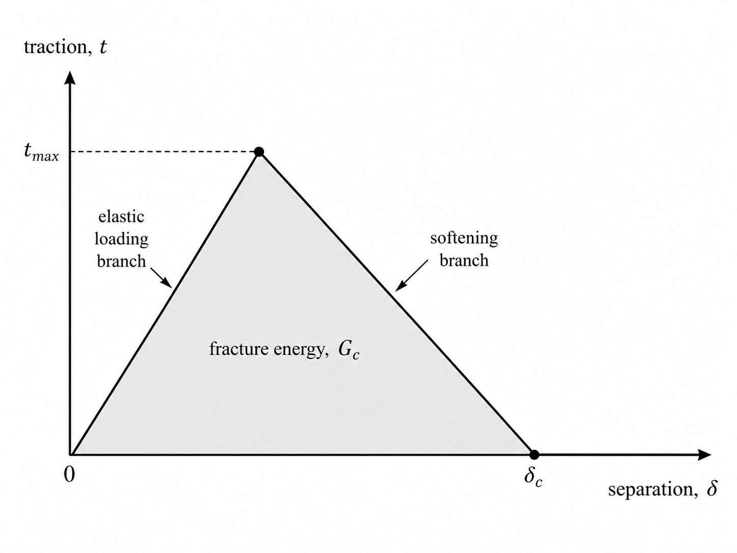
The peak traction controls strength.

The area under the curve controls fracture energy.

In ductile fracture, the cohesive response may depend on plastic deformation near the crack tip.

Some phase-field models incorporate cohesive-like degradation functions to better control both strength and fracture energy.

This is useful when one wants to match experimentally measured load-displacement curves and crack resistance behavior.

39. R-curve behavior

Ductile materials often show rising crack resistance.

This is called R-curve behavior.

Instead of a constant fracture toughness:

\[ G_c = \text{constant} \]

the resistance may increase with crack extension:

\[ G_R = G_R(\Delta a) \]

This occurs because plastic deformation around the crack tip evolves as the crack grows.

Brittle fracture often assumes a constant \(G_c\).

Ductile fracture may require evolving fracture resistance.

A phase-field model can represent this through:

plastic work contribution,
history-dependent fracture energy,
hardening-dependent damage resistance,
cohesive-zone-inspired laws.

40. Ductile fracture in metals

For metals, the common ductile fracture mechanisms include:

yielding,
strain hardening,
necking,
void nucleation,
void growth,
shear localization,
final coalescence.

A model that ignores plasticity may severely underpredict or misrepresent fracture behavior.

For example, a notched metal specimen may absorb a large amount of energy through plastic deformation before crack growth.

A brittle phase-field model would not capture this correctly.

41. Ductile fracture in polymers and soft materials

Ductile fracture in polymers and elastomers may involve:

large deformation,
viscoelasticity,
Mullins effect,
cavitation,
chain scission,
rate dependence,
temperature dependence.

A ductile or tough polymer may stretch significantly before failure.

For these materials, one may need to combine phase-field fracture with:

hyperelasticity,
viscoelasticity,
plasticity,
damage,
rate-dependent dissipation.

42. Ductile fracture in geomaterials and ice

Some geomaterials and ice-like materials may show both brittle and ductile behavior depending on:

temperature,
strain rate,
pressure,
confinement,
grain structure,
water pressure,
loading mode.

At low temperature or high strain rate, behavior may be more brittle.

At high temperature or slow deformation, behavior may be more ductile or creep-dominated.

For glacier ice, fracture may interact with:

viscous creep,
hydrofracture,
compressive overburden,
crevasse water pressure,
damage accumulation,
anisotropic fabric.

This means a simple brittle model may not always capture the full behavior.

43. Connection to creep fracture

Ductile fracture can be generalized further to creep fracture.

In creep fracture, damage evolves over time under sustained load.

The strain decomposition may involve:

\[ \varepsilon = \varepsilon^e + \varepsilon^p + \varepsilon^c \]

where:

\(\varepsilon^c\) is creep strain.

Damage may depend on:

creep strain,
creep work,
stress state,
time,
temperature.

This is especially relevant for high-temperature metals, polymers, and glacier ice.

44. Thermodynamic consistency

A ductile fracture model must satisfy the second law of thermodynamics.

The total dissipation should be nonnegative:

\[ \mathcal{D} = \mathcal{D}_p + \mathcal{D}_f \geq 0 \]

where:

\(\mathcal{D}_p\) is plastic dissipation,
\(\mathcal{D}_f\) is fracture dissipation.

Plastic dissipation:

\[ \mathcal{D}_p \geq 0 \]

Fracture dissipation:

\[ \mathcal{D}_f \geq 0 \]

This requirement constrains how the model can be formulated.

A model may look reasonable numerically but still be thermodynamically inconsistent if dissipation can become negative.

45. Implementation diagnostics

When implementing ductile phase-field fracture, output these fields:

Field	Purpose
\(d\)	crack/damage field
\(\bar{\varepsilon}^p\)	accumulated plastic strain
\(W_p\)	accumulated plastic work
\(\sigma_{\text{eq}}\)	von Mises stress
\(\sigma_m\)	mean stress
\(\eta\)	stress triaxiality
\(\theta_L\)	Lode angle
yield function \(f\)	checks plastic admissibility
plastic multiplier \(\Delta\lambda\)	shows active plastic flow
fracture driving force	shows where damage should grow
total plastic dissipation	energy check
total fracture dissipation	energy check

Useful debugging questions:

Does plasticity occur before ductile damage?
Does damage localize where plastic strain localizes?
Is the yield function close to zero in plastic zones?
Is the damage field irreversible?
Is energy dissipation nonnegative?
Does mesh refinement change the localization width?
Is stress triaxiality high where void growth is expected?

46. Common mistakes

Mistake 1: Treating ductile fracture as brittle fracture

If a ductile material undergoes large plastic deformation before failure, a purely brittle phase-field model is usually insufficient.

Mistake 2: Ignoring plastic dissipation

Ductile fracture absorbs energy through plastic flow.

Ignoring this can severely underestimate fracture resistance.

Mistake 3: Using equivalent plastic strain alone

Equivalent plastic strain is useful, but ductile fracture also depends on stress triaxiality and Lode angle.

Mistake 4: Forgetting damage irreversibility

As in brittle fracture:

\[ d_n \geq d_{n-1} \]

must be enforced.

Mistake 5: Not checking thermodynamic consistency

Plasticity and fracture must both dissipate energy.

Mistake 6: Using the wrong stress in the yield function

Be clear whether the yield condition uses degraded stress, effective stress, or undamaged stress.

Mistake 7: Ignoring finite strains

Many ductile fracture problems involve large deformation.

Small-strain models may fail in such cases.

47. Conceptual summary

Brittle fracture is mainly controlled by elastic energy release and fracture energy:

\[ G \geq G_c \]

Ductile fracture involves additional irreversible mechanisms:

\[ \text{plasticity} \]

\[ \text{void growth} \]

\[ \text{plastic dissipation} \]

\[ \text{stress-state-dependent failure} \]

A ductile phase-field model therefore couples:

\[ u \]

\[ \varepsilon^p \]

\[ \alpha \]

\[ d \]

where:

\(u\) is displacement,
\(\varepsilon^p\) is plastic strain,
\(\alpha\) is a hardening variable,
\(d\) is phase-field damage.

The key message is:

Ductile phase-field fracture is not just brittle phase-field fracture with different parameters; it requires coupling crack evolution to plasticity and ductile dissipation mechanisms.

48. Key terms

Term	Meaning
Ductile fracture	Fracture preceded by significant plastic deformation
Plastic strain	Permanent strain after unloading
Yield surface	Stress surface defining onset of plastic flow
Hardening	Increase of yield stress with plastic deformation
Equivalent plastic strain	Scalar measure of accumulated plastic deformation
Plastic work	Energy dissipated by plastic flow
Stress triaxiality	Ratio of mean stress to von Mises stress
Lode angle	Measure of deviatoric stress state
Void growth	Enlargement of microscopic voids under tensile stress
Void coalescence	Linking of voids to form a crack
Return mapping	Numerical algorithm for plastic constitutive update
R-curve	Crack resistance curve increasing with crack extension
Gradient plasticity	Plasticity model with length-scale regularization
Thermodynamic consistency	Requirement that total dissipation is nonnegative

49. Suggested references

Griffith, A. A. (1921). The phenomena of rupture and flow in solids. Philosophical Transactions of the Royal Society of London. Series A.
Gurson, A. L. (1977). Continuum theory of ductile rupture by void nucleation and growth: Part I — Yield criteria and flow rules for porous ductile media. Journal of Engineering Materials and Technology.
Tvergaard, V., & Needleman, A. (1984). Analysis of the cup-cone fracture in a round tensile bar. Acta Metallurgica.
Lemaitre, J. (1985). A continuous damage mechanics model for ductile fracture. Journal of Engineering Materials and Technology.
Ambati, M., Gerasimov, T., & De Lorenzis, L. (2015). Phase-field modeling of ductile fracture. Computational Mechanics.
Miehe, C., Aldakheel, F., & Raina, A. (2016). Phase field modeling of ductile fracture at finite strains. International Journal of Plasticity.
Miehe, C., Hofacker, M., & Welschinger, F. (2010). A phase field model for rate-independent crack propagation. Computer Methods in Applied Mechanics and Engineering.
Borden, M. J., Hughes, T. J. R., Landis, C. M., & Verhoosel, C. V. (2014/2016). Works on phase-field formulations for fracture in ductile materials.
Sur, A. S., and coauthors. (2025). A variational phase-field model for ductile fracture depending on stress triaxiality.
Anderson, T. L. (2017). Fracture Mechanics: Fundamentals and Applications. CRC Press.

This closes the sequence by showing how the same phase-field philosophy can be extended beyond brittle elastic fracture into elastoplastic and dissipative fracture processes.