Quick Start
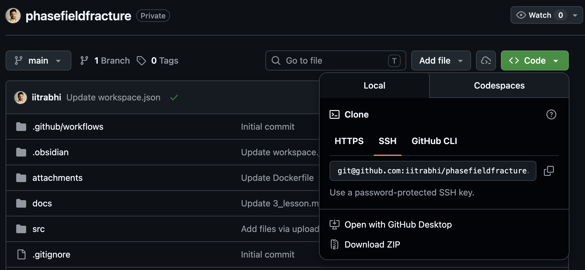
1. Download the Repository
Download or clone the supplied repository to your local machine.
https://github.com/iitrabhi/phasefieldfracture
2. Start the Docker Container
Open a terminal and navigate to the location where the repository was downloaded.
Replace path_of_the_supplied_folder with the full path to the downloaded repository and run:
docker run -p 8888:8888 \ -v path_of_the_supplied_folder:/root/codes/ \ -w /root/codes/ \ iitrabhi/fenics_notebook
For example:
docker run -p 8888:8888 -v ~/Storage/codes/2026/phasefieldfracture/:/root/codes/ -w /root/codes/ iitrabhi/fenics_notebook
3. Open JupyterLab
After the container starts, a URL similar to the one below will appear in the terminal:
http://127.0.0.1:8888/lab?token=...
Click (or copy and paste) this link into your browser to open JupyterLab.
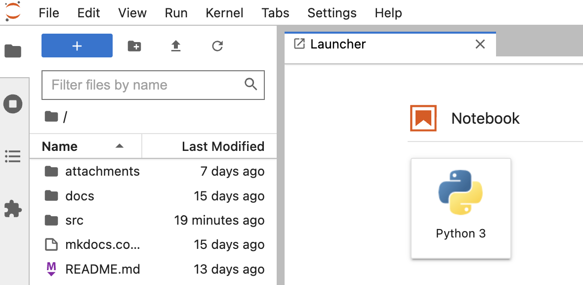
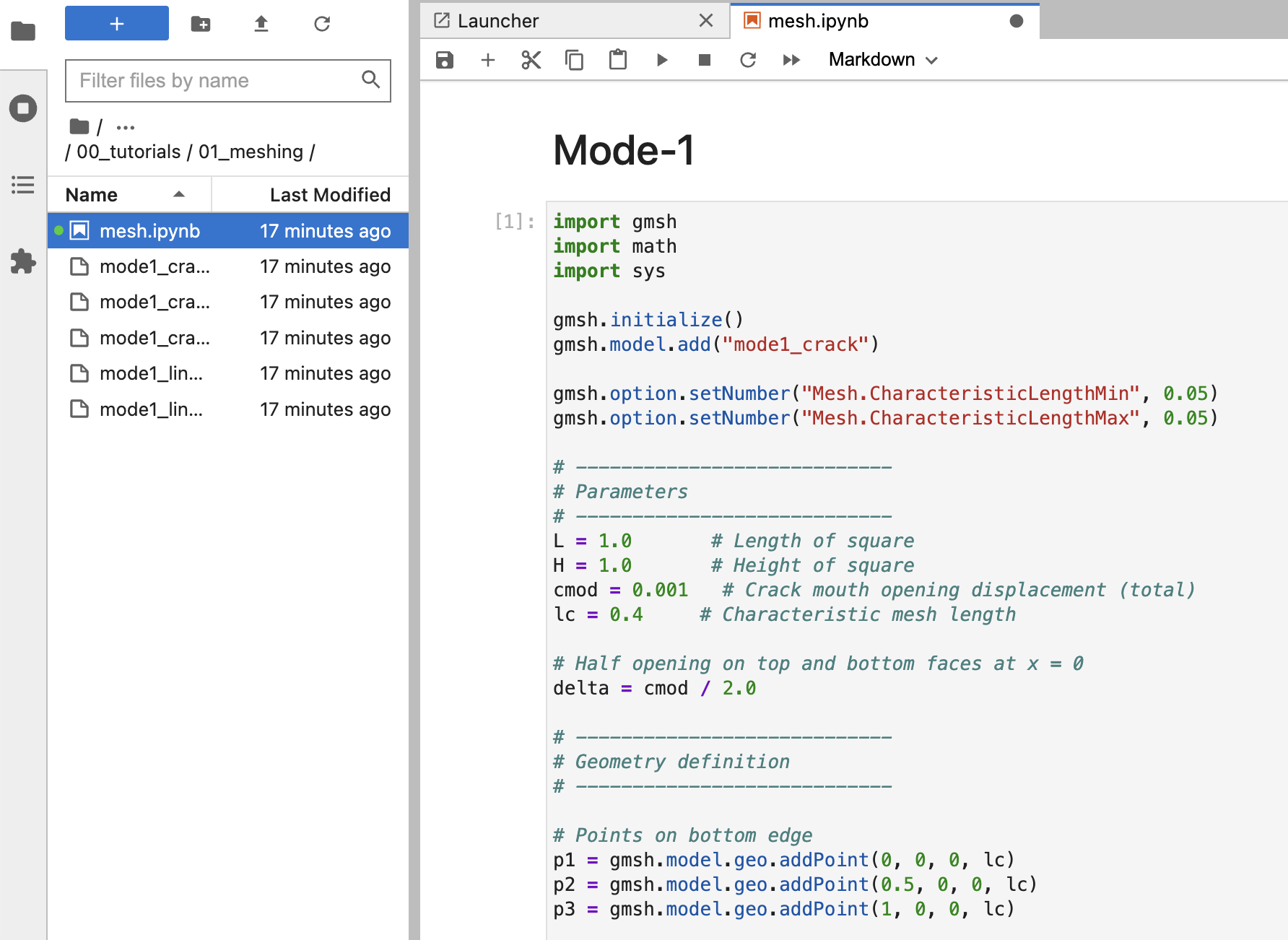
4. Run Notebook Cells
Open any notebook (.ipynb) file in JupyterLab.
To execute a cell: - Windows/Linux: Ctrl + Enter - macOS: Cmd + Enter
Run the cells sequentially from top to bottom.
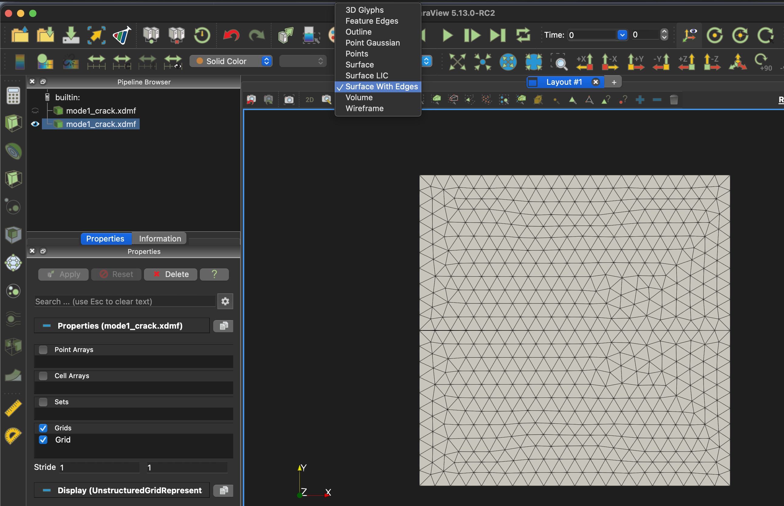
5. Visualize Results in ParaView
Simulation results are typically saved as .xdmf files.
- Locate the desired .xdmf file in JupyterLab.
- Double-click the file to open it in ParaView.
- Click Apply if prompted.
- Use the variable drop-down menu (e.g., displacement, phase field, stress, etc.) to select the quantity you would like to visualize.