Phase-Field Regularization of Griffith Fracture
Learning objectives
By the end of this lesson, you should be able to:
- Explain why sharp-crack Griffith fracture is difficult to implement directly.
- Understand the idea of replacing a sharp crack by a smooth damage field.
- Write the regularized crack surface density functional.
- Explain the role of the phase-field length scale \(\ell\).
- Understand how the Ambrosio-Tortorelli approximation connects to Griffith fracture.
- Interpret the main terms in the phase-field fracture energy.
- Understand the difference between AT1 and AT2 phase-field models.
1. Starting point: sharp Griffith fracture
In Griffith fracture, a cracked elastic body is described by two main unknowns:
and
where:
- \(u\) is the displacement field,
- \(\Gamma\) is the sharp crack set.
The total energy is written as
where:
- \(\Omega\) is the original body,
- \(\Omega \setminus \Gamma\) is the uncracked domain,
- \(\psi_e\) is the elastic strain energy density,
- \(G_c\) is the critical fracture energy,
- \(|\Gamma|\) is the crack length in 2D or crack surface area in 3D,
- \(W_{\text{ext}}\) is the work of external forces.
The fracture problem is then:
subject to crack irreversibility:
This means cracks can grow but cannot heal.
2. Why sharp cracks are difficult numerically
The sharp-crack formulation is physically elegant, but it is difficult to solve directly with standard finite element methods.
The reason is that the crack \(\Gamma\) is a discontinuity. As the crack grows, the computational domain changes:
This creates several numerical challenges:
- The mesh may need to conform to the crack path.
- The crack path is usually not known in advance.
- Crack branching is difficult to handle.
- Crack merging requires special algorithms.
- Crack nucleation requires an additional criterion.
- The displacement field is discontinuous across the crack.
- Computing \(|\Gamma|\) requires explicit crack geometry tracking.
For example, if a crack curves through the body, one may need remeshing or special enrichment functions. If the crack branches into multiple cracks, explicit tracking becomes even more complicated.
The phase-field approach avoids this by replacing the sharp crack with a smooth field.
3. Main idea of phase-field regularization
Instead of representing a crack as a sharp geometric surface, phase-field fracture introduces a scalar damage variable:
where:
- \(d = 0\) means intact material,
- \(d = 1\) means fully broken material,
- \(0 < d < 1\) means partially damaged material.
The crack is no longer represented as a discontinuity. Instead, it is represented as a narrow diffused zone.
Sharp crack:

intact material | crack | intact material

Phase-field crack:

intact material → damaged zone → intact material
In a one-dimensional view, the damage field may look like this:
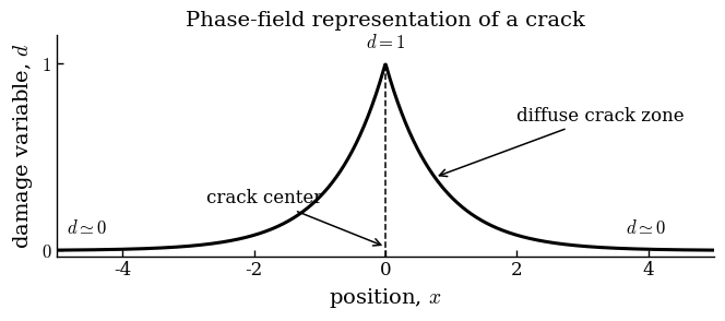
The width of this damaged zone is controlled by a length scale parameter:
This parameter is called the phase-field length scale or regularization length.
4. Regularized crack surface density
In sharp Griffith fracture, the fracture energy is
where \(|\Gamma|\) is the crack measure.
In phase-field fracture, we approximate \(|\Gamma|\) by an integral over the whole domain:
where \(\gamma_\ell(d,\nabla d)\) is the crack surface density function.
A common choice is the AT2 crack density:
Therefore,
The fracture energy becomes
This is the regularized version of the Griffith crack surface energy.
5. Meaning of the two crack-density terms
The regularized crack density is
It contains two terms.
Damage magnitude term
This term penalizes the amount of damage.
If \(d\) becomes large over a wide region, this term increases the fracture energy.
So the model does not allow damage to spread everywhere for free.
Damage gradient term
This term penalizes rapid spatial changes in damage.
If \(d\) jumps abruptly from 0 to 1, then \(|\nabla d|\) becomes large.
So this term smooths the crack over a finite width.
Together, these two terms create a localized but smooth damage band.
6. Role of the length scale \(\ell\)
The parameter \(\ell\) controls the width of the diffused crack.
Small \(\ell\):
- gives a sharper crack,
- gives a narrower damage zone,
- more closely approximates the sharp Griffith crack,
- requires a finer mesh.
Large \(\ell\):
- gives a wider crack band,
- makes the solution smoother,
- is easier to resolve numerically,
- may artificially broaden the fracture process zone.
A rough practical requirement is:
where \(h\) is the element size.
In practice, many simulations use several elements across the damage band.
A common numerical rule is:
or even
depending on the desired accuracy.
Warning
The length scale \(\ell\) is not just a numerical parameter in all models.
In some settings, it may represent a material length scale related to the fracture process zone. In other settings, it is mainly a regularization parameter that must be chosen carefully and resolved by the mesh.
7. From sharp-crack energy to phase-field energy
The sharp Griffith energy is
The phase-field approximation replaces \(\Gamma\) by \(d\):
where:
- \(u\) is the displacement field,
- \(d\) is the phase-field damage variable,
- \(g(d)\) is the degradation function,
- \(\psi_e\) is the elastic strain energy density,
- \(G_c\) is the fracture energy,
- \(\ell\) is the regularization length.
This is the basic energy functional of phase-field fracture.
8. Degradation function
The degradation function \(g(d)\) reduces material stiffness as damage grows.
A common choice is
where \(k\) is a very small positive number.
The function has the following behavior:
- when \(d = 0\), \(g(d) \approx 1\),
- when \(d = 1\), \(g(d) \approx k\).
So:
d = 0  → intact material  → full stiffness
d = 1  → broken material  → almost zero stiffness
The small number \(k\) is called a residual stiffness.
It prevents the stiffness matrix from becoming exactly singular in fully broken regions.
Usually,
For example,
or
may be used depending on the problem.
9. Why not set stiffness exactly to zero?
If \(d = 1\) and \(g(d) = 0\), then the material at the crack becomes completely stress-free.
Physically, this makes sense.
Numerically, however, this can cause problems.
If some elements have exactly zero stiffness, the global stiffness matrix can become singular. Then the finite element solver may fail.
To avoid this, we use
with a small \(k > 0\).
This keeps a tiny amount of stiffness in fully damaged regions.
Note
The value of \(k\) should be small enough that it does not noticeably affect the physical solution, but large enough to avoid severe numerical singularity.
10. AT2 model
The most common crack density function is the AT2 model:
The corresponding fracture energy is
AT2 is smooth and easy to implement.
However, AT2 has an important feature:
Damage can begin gradually before a sharp critical stress is reached.
This means AT2 does not always produce a strict elastic stage unless the formulation is modified.
11. AT1 model
Another common model is AT1.
The AT1 crack density is commonly written in normalized form as
The corresponding fracture energy is
The key difference is that AT1 uses \(d\), while AT2 uses \(d^2\).
AT1 has a more threshold-like damage initiation behavior.
In simple settings, AT1 can produce an initial purely elastic regime before damage starts.
12. Comparing AT1 and AT2
| Feature | AT1 | AT2 |
|---|---|---|
| Crack density term | \(d/\ell\) | \(d^2/(2\ell)\) |
| Damage onset | Has a finite threshold | Damage can start gradually |
| Smoothness | Less smooth near \(d=0\) | Smooth |
| Implementation | Slightly more delicate | Very common and simple |
| Elastic stage | Usually yes | Not strictly, unless modified |
| Historical use | Widely used | Very widely used |
Both AT1 and AT2 approximate Griffith fracture, but they differ in damage initiation behavior and numerical properties.
13. One-dimensional crack profile intuition
To understand the role of \(\ell\), consider a one-dimensional crack centered at \(x=0\).
For the AT2 model, an idealized damage profile has the form
This profile is maximum at the crack center:
and decays away from the crack.
At a distance of a few multiples of \(\ell\), the damage becomes very small.
For example:
- at \(x = \ell\), \(d \approx e^{-1} \approx 0.37\),
- at \(x = 2\ell\), \(d \approx e^{-2} \approx 0.14\),
- at \(x = 3\ell\), \(d \approx e^{-3} \approx 0.05\).
So the visible damaged region has width of a few times \(\ell\).
14. Gamma-convergence idea
The phase-field approximation is not just an engineering trick.
Mathematically, the regularized energy is connected to sharp-crack Griffith fracture through a concept called Gamma-convergence.
Informally:
This means that as the length scale becomes very small, the minimizers of the phase-field problem approach minimizers of the sharp-crack problem.
The Ambrosio-Tortorelli functional is a foundational mathematical result behind this type of approximation.
For practical purposes, you can remember:
Phase-field fracture replaces the difficult crack-surface measure \(|\Gamma|\) by a smooth volumetric integral that approaches the sharp crack energy as \(\ell \to 0\).
15. Crack irreversibility
A fracture model must prevent crack healing.
In sharp-crack Griffith fracture, irreversibility is written as
In phase-field fracture, this becomes
or in rate form,
This means:
- damage can increase,
- damage can stay the same,
- damage cannot decrease.
Without this condition, the model could predict that cracks heal during unloading, which is not physical for brittle fracture.
16. Mesh requirements
The damage band must be resolved by the mesh.
If the mesh is too coarse compared to \(\ell\), then:
- the crack may appear too wide or too narrow,
- the fracture energy may be inaccurate,
- the peak load may be mesh-dependent,
- the crack path may be affected by mesh bias.
A practical guideline is:
or preferably
where \(h\) is the local element size.
For adaptive mesh refinement, a natural strategy is to refine where:
- \(d\) is large,
- \(|\nabla d|\) is large,
- the crack-driving energy is high,
- the mesh size \(h\) is not small enough compared to \(\ell\).
17. Why phase-field fracture is attractive
Phase-field fracture has several advantages.
No explicit crack tracking
The crack path is represented by \(d\), so we do not need to explicitly track crack geometry.
Natural crack branching
Cracks can branch because \(d\) evolves over the full domain.
Natural crack merging
Multiple cracks can merge without special algorithms.
Standard finite element implementation
The problem can be solved using standard finite element spaces for \(u\) and \(d\).
Energy-based formulation
The model remains connected to Griffith's energy principle.
18. Main limitations
Phase-field fracture is powerful, but it also has limitations.
Length-scale sensitivity
The solution may depend on \(\ell\), especially for finite values of \(\ell\).
Mesh resolution cost
Small \(\ell\) requires fine meshes, making 3D simulations expensive.
Damage before failure
Some models, especially AT2, may show gradual damage evolution before macroscopic crack growth.
Tension-compression ambiguity
Different energy splits can produce different results.
Parameter calibration
Choosing \(G_c\), \(\ell\), and degradation functions requires care.
19. Conceptual summary
Sharp Griffith fracture uses the energy
Phase-field fracture replaces the sharp crack \(\Gamma\) with a smooth scalar field \(d\):
The main idea is:
Replace the sharp crack surface measure \(|\Gamma|\) by a smooth volumetric integral involving \(d\) and \(\nabla d\).
This allows cracks to nucleate, propagate, branch, and merge without explicitly tracking crack geometry.
20. Key terms
| Term | Meaning |
|---|---|
| Sharp crack | A discontinuous crack surface or crack line |
| Phase-field | Smooth scalar variable used to represent cracks |
| Damage variable \(d\) | Field where \(d=0\) is intact and \(d=1\) is broken |
| Regularization length \(\ell\) | Parameter controlling diffused crack width |
| Crack density function \(\gamma_\ell\) | Volumetric approximation of crack surface density |
| AT1 model | Phase-field model with linear damage term |
| AT2 model | Phase-field model with quadratic damage term |
| Degradation function \(g(d)\) | Function reducing stiffness as damage increases |
| Residual stiffness \(k\) | Small stiffness left in broken regions for numerical stability |
| Gamma-convergence | Mathematical notion connecting regularized and sharp-crack energies |
| Irreversibility | Condition that damage cannot decrease |
21. Suggested references
- Griffith, A. A. (1921). The phenomena of rupture and flow in solids. Philosophical Transactions of the Royal Society of London. Series A.
- Ambrosio, L., & Tortorelli, V. M. (1990). Approximation of functional depending on jumps by elliptic functional via Gamma-convergence. Communications on Pure and Applied Mathematics.
- Francfort, G. A., & Marigo, J.-J. (1998). Revisiting brittle fracture as an energy minimization problem. Journal of the Mechanics and Physics of Solids.
- Bourdin, B., Francfort, G. A., & Marigo, J.-J. (2000). Numerical experiments in revisited brittle fracture. Journal of the Mechanics and Physics of Solids.
- Bourdin, B., Francfort, G. A., & Marigo, J.-J. (2008). The variational approach to fracture. Journal of Elasticity.
- Miehe, C., Hofacker, M., & Welschinger, F. (2010). A phase field model for rate-independent crack propagation. Computer Methods in Applied Mechanics and Engineering.
- Pham, K., Amor, H., Marigo, J.-J., & Maurini, C. (2011). Gradient damage models and their use to approximate brittle fracture. International Journal of Damage Mechanics.
At this point, the model has an energy functional in terms of displacement and damage. The next step is to take variations of that energy to obtain the governing equations.