How to get production-ready plots from python.

The problem

I would love to have production-ready plots directly from python.

The Solution

First of all download the following dependencies

pip install numpy
pip install matplotlib
pip install svglib
pip install reportlab

You also need to have latex installed on your system. Check the complete workflow for installation here.

We are now going to go step by step into understanding the complete workflow of building a plot for your scientific work.

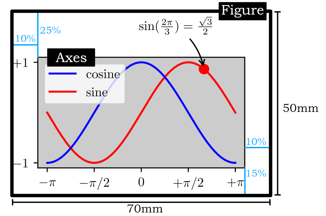
Figure: It is the complete image that you get out of matplotlib
Axes: It is the actual plotting area as seen in the grey background in the picture below.

matplotlib-plot-dimensions

Selecting the proper plot size

It is very important to understand that figures and plots are a way of communicating your ideas and findings to a bigger community. Typically most of the research documents are made for an A4 size sheet of paper. The width of an A4 size paper is 210mm, take out the 30mm right and left margin and you are left with 150mm of usable space. That is the space that you should always use while designing your figures. Thus, you only have two width options

150mm if you are designing for full width
70mm if you are designing for a two-column layout

It is inside this space constraint that you have to draw. Thus, we will begin by setting up the space inside matplotlib

import matplotlib.pyplot as plt
import numpy as np

mm = 1/25.4  # millimeters in inches
fig = plt.figure(figsize=(70*mm,50*mm), dpi=200)  # create a figure object
fig.subplots_adjust(left=0.1, right=0.9, top=0.75, bottom=0.15)
ax = fig.add_subplot(1, 1, 1)  # create an axes object in the figure
plt.close() # Closes the plot in jupyter while creating axes

plt.figure command will set the size of the figure and with the help of plt.subplots_adjust we can adjust the padding around the plot as a percentage of the width and height of the figure. The arguments left, right, bottom and top are fractional units (of the total figure dimensions).

Tell matplotlib to use LaTeX

Now we will tell python to use latex fonts and also set the font size to 10. This is the font size that we use for the main content of our article. It is very important to have consistency in the font size and your figure font size should always match your article font size.

plt.rcParams.update({
    "text.usetex": True,
    "font.family": "serif",
    "font.size": 10,
    "pdf.fonttype":42})

The pdf.fonttype option will force python to use TrueType fonts

Plot

Now the figure is ready to plot and save as a pdf. The figure will have the correct physical dimensions and the correct font size.

X = np.linspace(-np.pi, np.pi, 256,endpoint=True)
C,S = np.cos(X), np.sin(X)

ax.plot(X, C, color="blue", linewidth=1.5)
ax.plot(X, S, color="red", linewidth=1.5)

Export the file to pdf

If you do not wish to edit your file you can now directly export it as a pdf using

fig.savefig("plot.pdf", format="pdf")

But, if you wish to edit your file in a vector-based editing program then the file generated from the above command would result in the wrong rendering of text. To prevent this we can save the figure as SVG and then convert that to pdf. Writing to SVG will convert the text to a path and thus it will render properly in a vector-based editing program. To do that use the following code

fig.savefig("plot.svg", format="svg")

from svglib.svglib import svg2rlg
from reportlab.graphics import renderPDF

drawing = svg2rlg("plot.svg")
renderPDF.drawToFile(drawing, "plot.pdf")

Complete code

import matplotlib.pyplot as plt
import numpy as np
from svglib.svglib import svg2rlg
from reportlab.graphics import renderPDF

plt.rcParams.update({
    "text.usetex": True,
    "font.family": "serif",
    "font.size": 10,
    "pdf.fonttype":42})

mm = 1/25.4  # millimeters in inches
fig = plt.figure(figsize=(70*mm,50*mm), dpi=200)  # create a figure object
fig.subplots_adjust(left=0.1, right=0.9, top=0.75, bottom=0.15)
ax = fig.add_subplot(1, 1, 1)  # create an axes object in the figure
plt.close() # Closes the plot in jupyter while creating axes

X = np.linspace(-np.pi, np.pi, 256,endpoint=True)
C,S = np.cos(X), np.sin(X)

ax.plot(X, C, color="blue", linewidth=1.5, linestyle="-", label="cosine",
         zorder=-1)
ax.plot(X, S, color="red", linewidth=1.5, linestyle="-",  label="sine",
         zorder=-2)

ax.set_xlim(X.min()*1.1, X.max()*1.1)
ax.set_xticks([-np.pi, -np.pi/2, 0, np.pi/2, np.pi],
           [r'$-\pi$', r'$-\pi/2$', r'$0$', r'$+\pi/2$', r'$+\pi$'])

ax.set_ylim(C.min()*1.1,C.max()*1.1)
ax.set_yticks([-1, +1],
           [r'$-1$', r'$+1$'])

ax.legend(loc='upper left', frameon=True)

t = 2*np.pi/3
ax.scatter([t,],[np.sin(t),], 50, color ='red')
ax.annotate(r'$\sin(\frac{2\pi}{3})=\frac{\sqrt{3}}{2}$',
             xy=(t, np.sin(t)),  xycoords='data',
             xytext=(-50, +30), textcoords='offset points',
             arrowprops=dict(arrowstyle="->", connectionstyle="arc3,rad=-.2"))

for label in ax.get_xticklabels() + ax.get_yticklabels():
    label.set_bbox(dict(facecolor='white', edgecolor='None', alpha=0.65 ))

fig.savefig("plot.svg", format="svg")
drawing = svg2rlg("plot.svg")
renderPDF.drawToFile(drawing, "plot.pdf")